Table
Ranges can be converted into tables.
Tables make it easier to structure and organize data.
Note: The filter function is similar to a table. The filter can be better used if the only function needed is to sort and filter data.
Tables connect cells in a range and put it into a fixed structure.
The cells in the table range share the same formatting.
Note: Tables can be used to prepare data for charts and pivot tables.
Tables allow for options such as:
- Sort & Filter
- Formatting
- AutoFilling
Note: Tables can be converted back to range.
Example
Formatting a range into a table will give it a new form with a fixed structure. Tables open access to new functionality such as: filtering, automations and styling.
Example (Converting a Range to Table)
How to convert range to table, step by step.
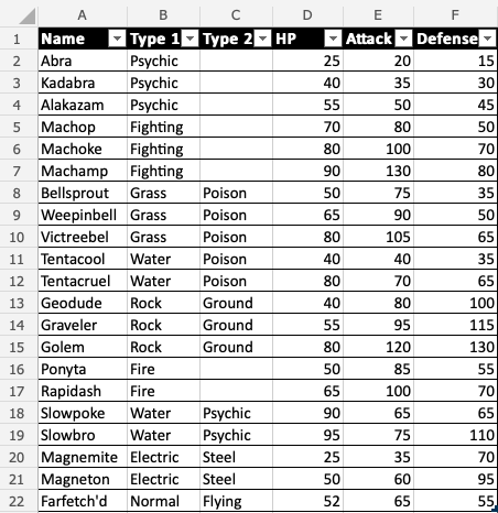
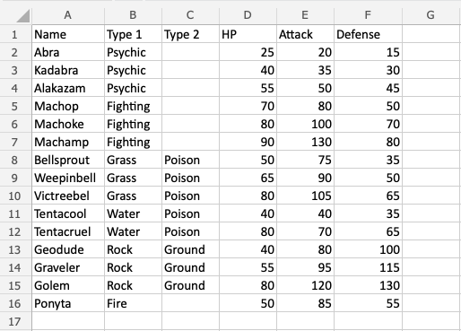
Copy the values to follow along:
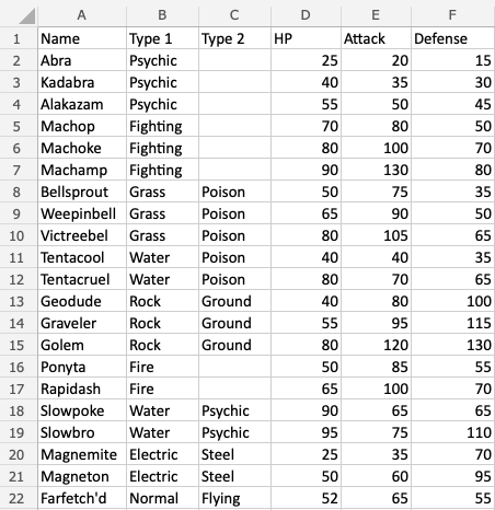
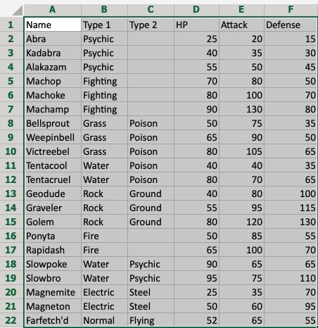
- Select range
A1:F22
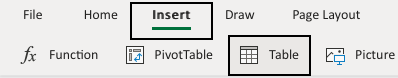
- Click Insert, then Table (
 ), in the Ribbon.
- Click OK
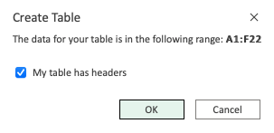
Note: The range (A1:F22) already has headers in row 1. Unchecking the “My table has headers” option allows you to create a dedicated header if you do not already have it.
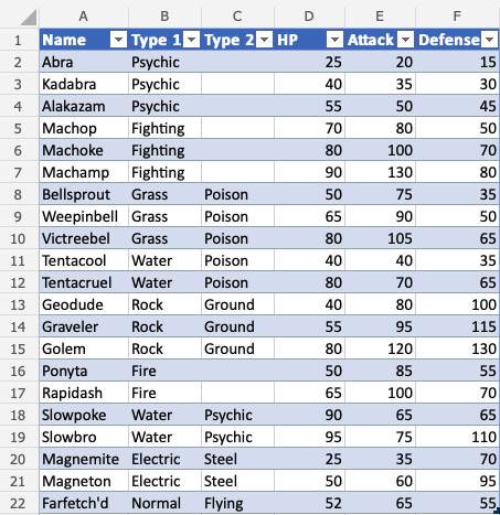
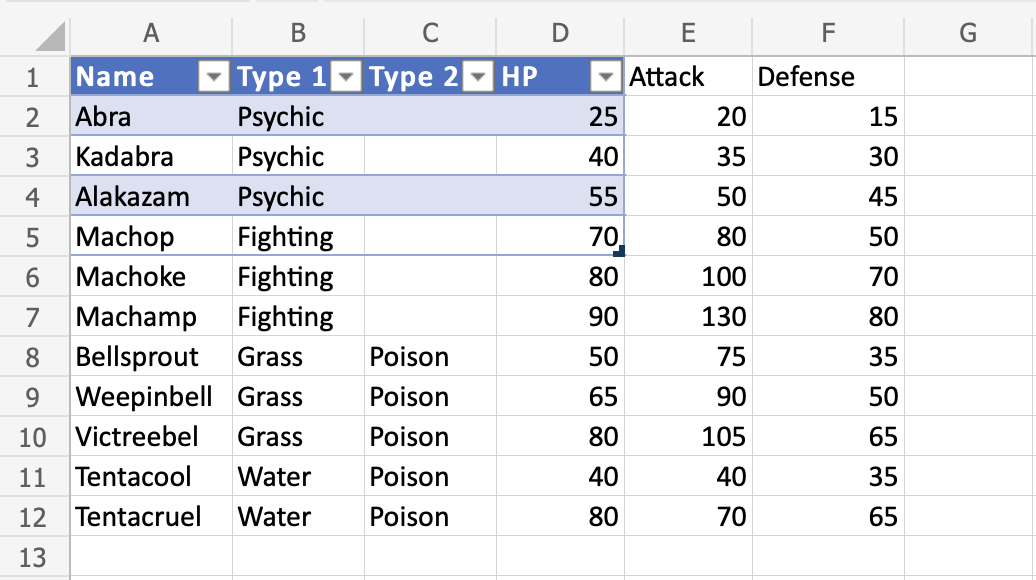
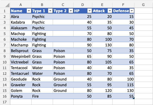
Good job! The range A1:F22 was successfully converted from range to table.
The range is now a fixed table structure and new options such as sorting and filtering are now enabled.
Applying the filter keeps the relationship between the columns while sorting and filtering.
Excel Table Design
Table Design
Tables can be customized and styled in a few clicks.
Converting a range into a table gives access to a menu called “Table Design”.
![]()
The menu appears when selecting a cell in the table’s range.
This menu has options and commands such as:
- Resize
- Remove duplicates
- Convert to range
- Style options (Total row, Header row, Banded row etc..)
- Formatting
Table Name
Excel gives tables default names such as: Table 1, Table 2, Table 3 and so on.
Note: Tables cannot be renamed in the Excel online version.
The name of the table can be found in the Table Design tab
- Select the table
- Click the Table design menu
- See the name input field
![]()
Note: It is useful to know the table names when you have many tables in a workbook and are referring to them in formulas.
In the next chapter you will learn about resizing a table.
Excel Table Resizing
Table Resizing
The size of a table can be changed.
Resizing is to increase or decrease the range of the table.
There are three ways to resize a table
- Resize table command
- Drag to resize
- Adding headers
Note: Resizing will continue formatting and formulas. This will be covered in a later chapter.
Resize Table Command
The resize table command allows you to change the size of the table by entering a range.
For example by entering A1:D10.
The command is found in the Ribbon under the Table Design tab.
![]()
Example – Resizing a Table
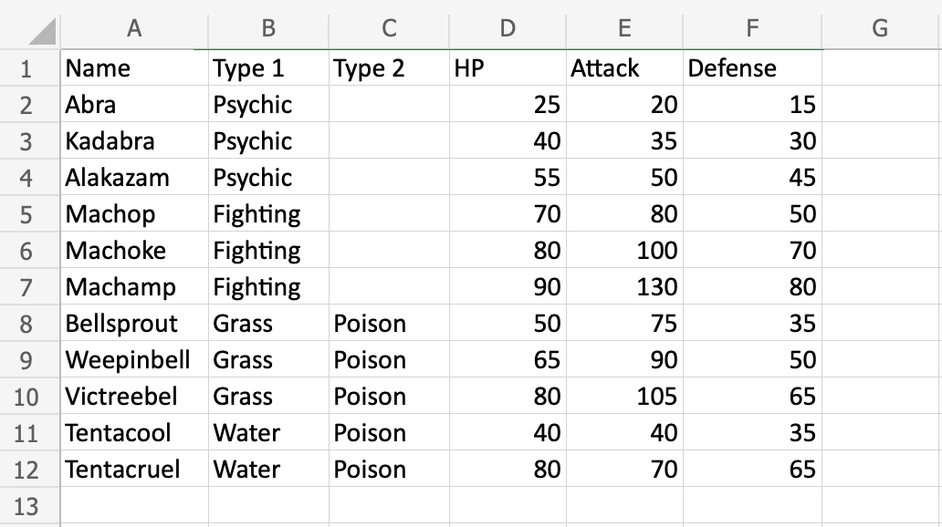
Convert the range into a table.
Lets resize the table from range A1:F12 to A1:F20
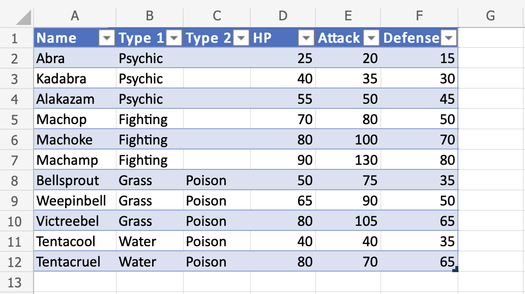
- Select the table
- Click the Table Design menu
![]()
- Click the Resize Table command (
 )
)
Clicking the Resize Table command allows you to set a new range for the table.
- Click the range input field
- Type the new range,
A1:F20
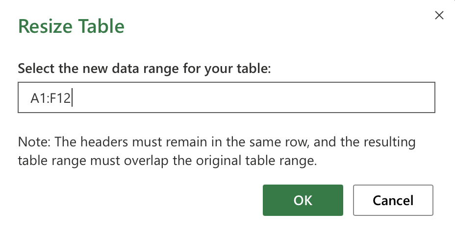
- Click OK
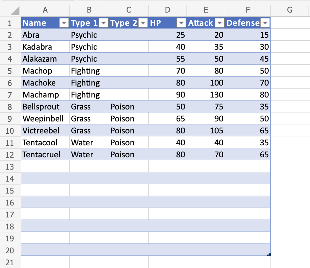
Great! The table has been resized to from A1:F12 to A1:F20.
Drag to Resize
The table can be resized by dragging its corner.
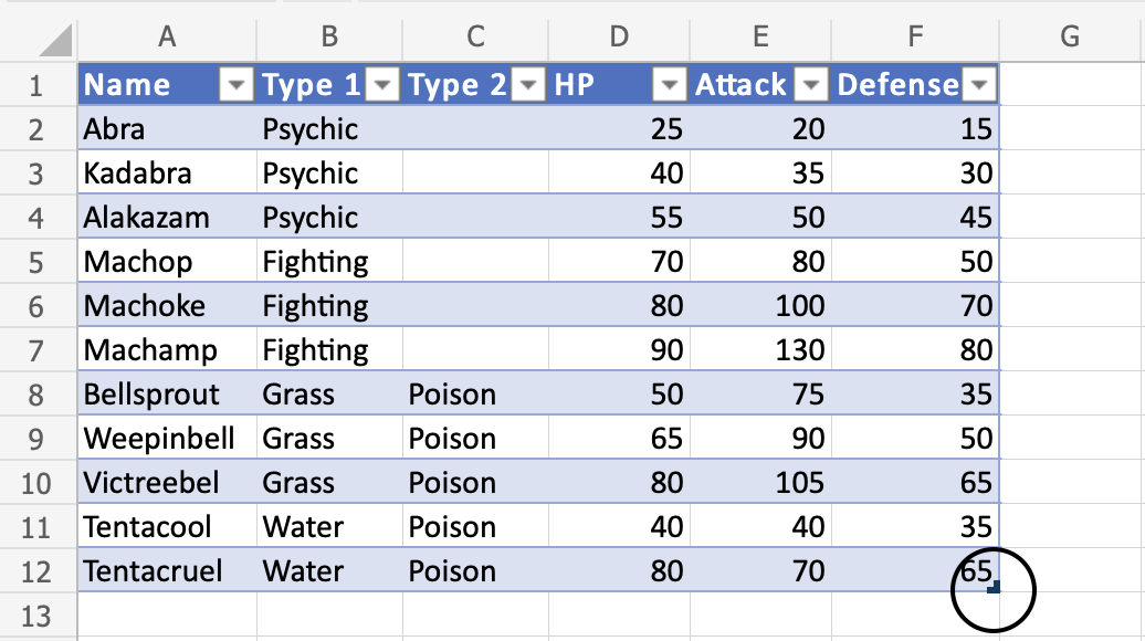
Example – Dragging to Resize, Smaller
Change the tables size from A1:F12 to A1:D5
- Press and hold the bottom right corner of the table (
 )
)
- Move the pointer, marking the range
A1:D5
The table range has been changed from A1:F12 to A1:D5.
Note: Cells outside of the table range are no longer included in the table. The connection between the cells created by the table is broken and they no longer have the table formatting.
Let’s try to sort the Pokemon by their names to see what happens.
- Click the filter option in
A1
- Sort by Ascending (A-Z)
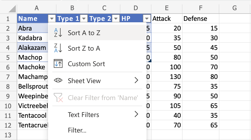
The filter option only includes the Pokemon in the tables range (A1:A5). The connection to the cells outside of the table is broken.
Lets resize again, this time bigger.
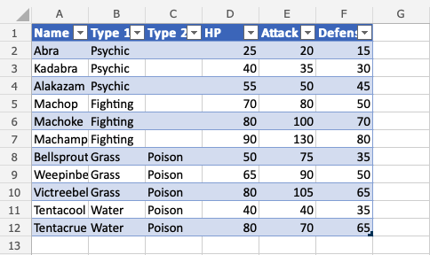
Example – Dragging to Resize, Bigger
Change the tables size from A1:D5 to A1:G13
- Press and hold the bottom right corner of the table ()
- Move the pointer to mark
A1:G13
The table range has been changed from A1:D5 to A1:G13.
The rest of the cells are now included again, and the connection between the cells is back.
Let’s try to filter the Pokemon by their names to see what happens.
- Click the filter option in
A1
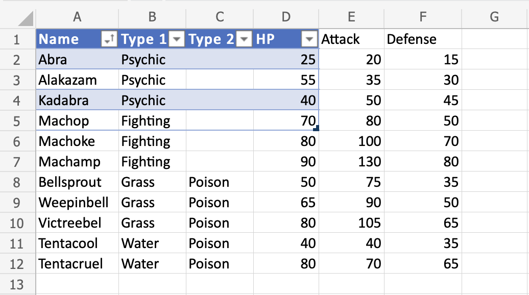
- Sort by Ascending (A-Z)
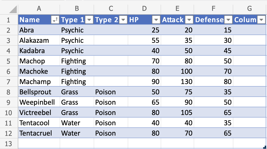
Nice! The table has successfully sorted the Pokemon in the range A1:A12 by their names.
Oh wait. Something has changed. A new column (G) has appeared…
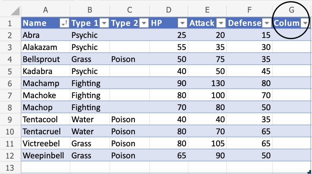
Increasing the table size will continue the formatting, formulas and add new columns.
Note: It will not overwrite the name for existing headers. It will use the value that is typed in the header cell.
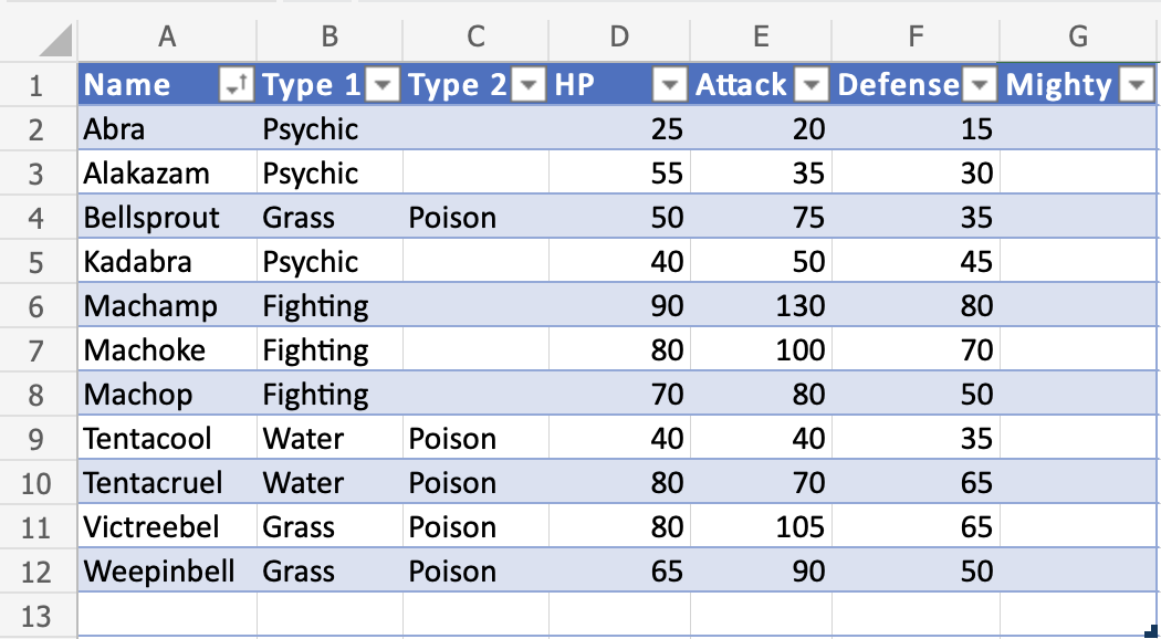
The header name can be changed.
- Double click
G1
- Delete the text
- Type “Mighty” to
G1
Another Example – Resize By Adding Columns
The table is automatically increased when new headers next to the table are added.
- Type “Mew” to
H1 - Hit enter
- Type “Two” to
I1 - Hit enter
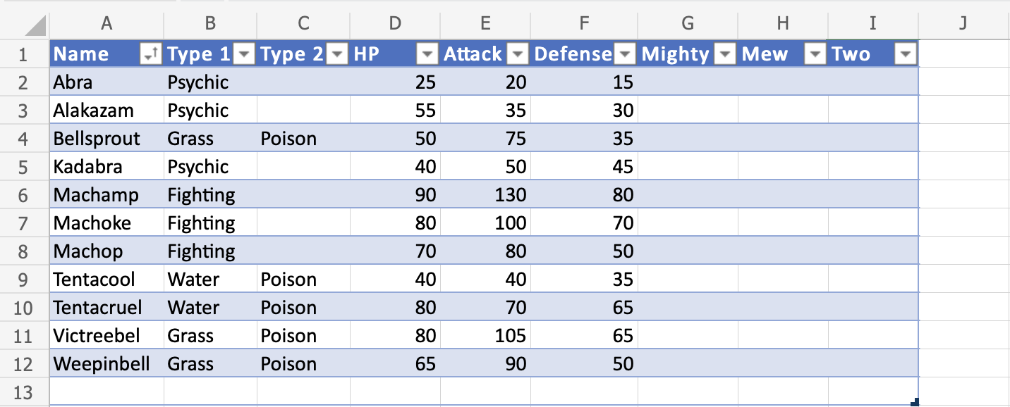
New columns with appropriate rows are automatically added when new headers are typed.
In the next chapter you will learn about removing duplicates.
Excel Removing Duplicates
Removing Duplicates
Excel has a command to remove duplicates in tables.
Note: Duplicates are extra copies of values.
Removing duplicates are helpful when cleaning a dataset and you do not want to include copies.
The Remove Duplicate function is found in the Ribbon under the Table Design tab.
![]()
The command allows you to specify the column where you want to find and remove duplicates.
Once applied it will return the number of deleted values and how many unique ones that remains.
Note: The remove duplicate command will not ask for which duplicates to delete. Make sure that it does not delete useful data.
Examples – Remove Duplicates command
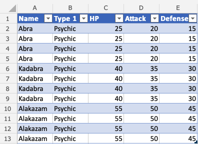
Lets try an example removing the duplicate Pokemon in the range A1:E13
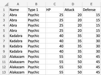
Convert the range into a table.
- Select the table
- Click the Table Design tab (
 )
)
- Click the Remove Duplicates command (
 )
)
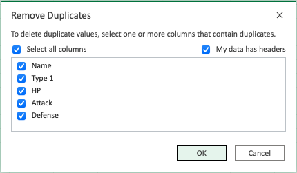
- Leave all columns checked
- Click OK
Note: Unchecking a column means that it will not remove duplicates for that column.
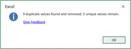
The command returns the number of found and removed duplicates and how many unique ones that remain.
- Click OK
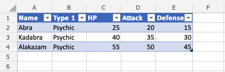
The remove duplicates command has successfully removed the 9 duplicate Pokemon from the range and the table has been resized accordingly. The remaining 3 values are unique.
Excel Converting a Table to Range
Tables can be reversed and converted back to range.
Tables can be converted to ranges by selecting a cell in the table range and clicking on the Convert to Range command.
The command to convert to range is found in the Table Design tab, in the Tools group.
![]()
Example – Convert Table to Range
Type or copy the values to follow the example.
Convert the range into a table.
- Select a cell in the table range (
A1:F16)
- Click the Design Table tab ()
- Click the Convert to Range command (
 )
)
The table is now converted into a range and it no longer has the table options available.
Note: The cell formatting is kept for the range after the conversion.
Excel Table Style
Table Style
Excel has many ready to use styles which can be applied for tables.
Table styles is to change the appearance of the table.
It can be changed to:
- Make it easier to read and understand
- Make it look better
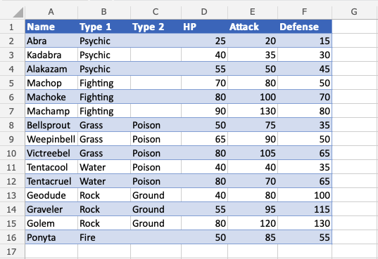
The table style is Blue, Table Style Medium 2 by default.
Example: Blue, Table Style Medium 2, which is how the default looks like.
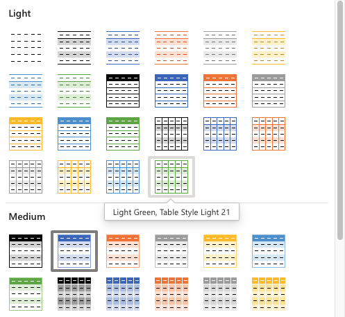
Excel has three main categories for Table styles:
- Light; Light colors, more white space
- Medium; Medium colors, medium white space
- Dark; Dark colors, less white space
The table style can be applied in a few steps.
Example – Applying Light Style
Type or copy the values to follow along:
Convert the range into a table.
- Select a cell in the table range
- Click the Design Table tab ()
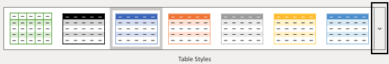
- Click on the Table Styles option button
Note: The Table Style that is already applied has a green rectangle around it. In this case Blue, Table Style Medium 2.
Clicking the Table Style option button opens a menu with different style options.
Here the three categories are presented; Light, Medium and Dark
- Click on the Light, Green, Table Style Light 21. Found in the Light category.
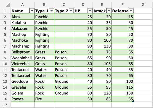
Well done! The formatting of the table has changed to the light green style.
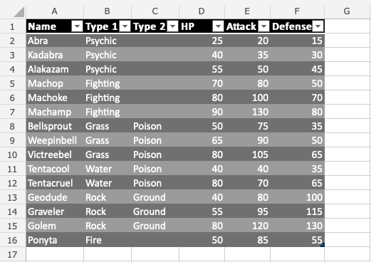
Apply Gray, Table Style Dark 4. Found in the Dark category.
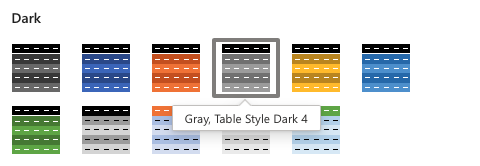
Did you make it?
Note: Get familiar with the Table Styles. Try different options to see how they look.