Highlight Cell Rules
Highlight Cell Rules is a premade type of conditional formatting in Excel used to change the appearance of cells in a range based on your specified conditions.
The conditions are rules based on specified numerical values, matching text, calendar dates, or duplicated and unique values.
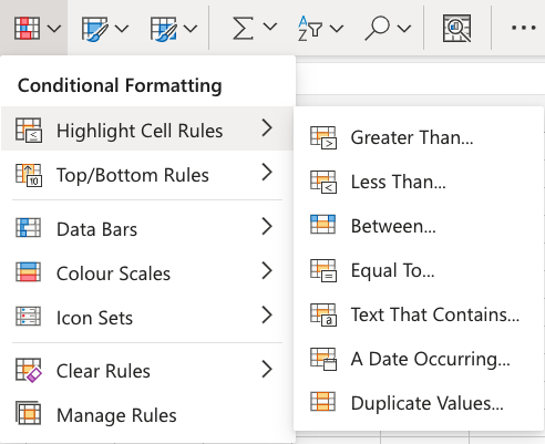
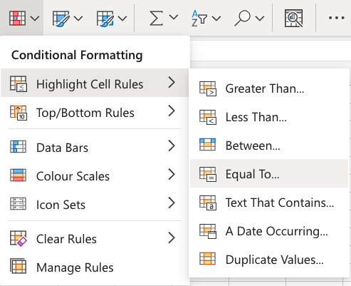
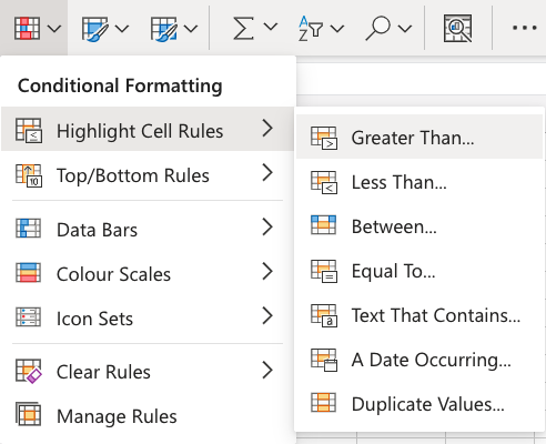
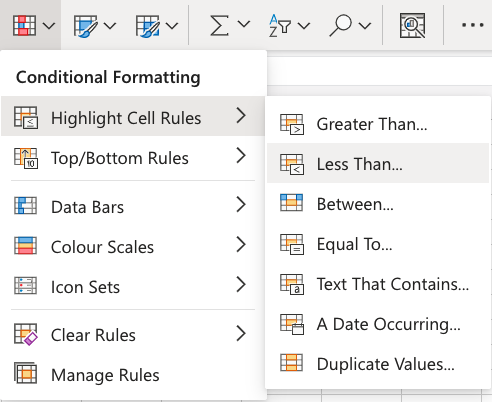
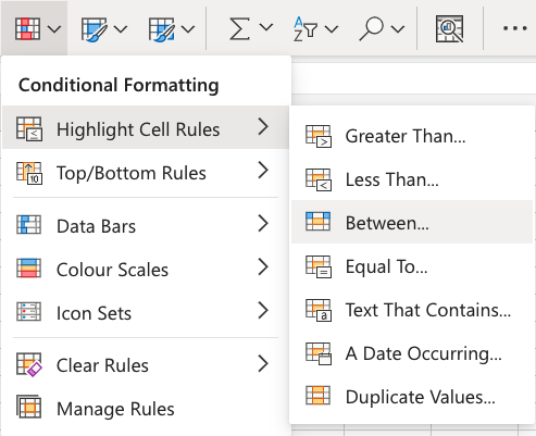
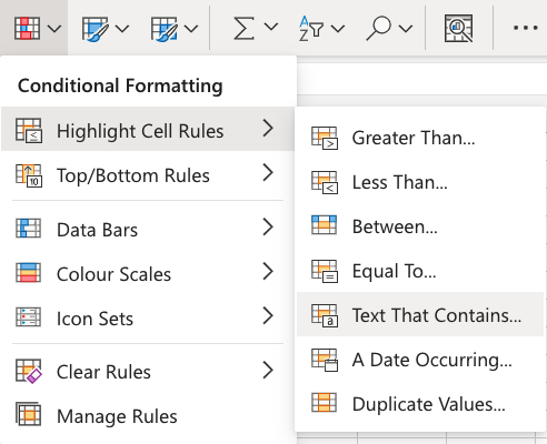
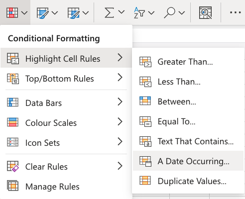
Here is the Highlight Cell Rules part of the conditional formatting menu:
Appearance Options
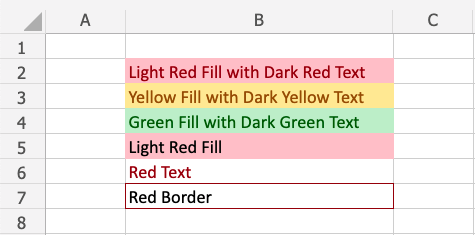
The web browser version of Excel offers the following appearance options for conditionally formatted cells:
- Light Red Fill with Dark Red Text
- Yellow Fill with Dark Yellow Text
- Green Fill with Dark Green Text
- Light Red Fill
- Red Text
- Red Border
Here is how the options look in a spreadsheet:
Cell Rule Types
Excel offers the following cell rule types:
- Greater Than…
- Less Than…
- Between…
- Equal To…
- Text That Contains…
- A Date Occurring…
- Duplicate/Unique Values
Highlight Cell Rule Example
The “Equal To…” Highlight Cell Rule will highlight a cell with one of the appearance options based on the cell value being equal to your specified value.
The specified value could be a particular number or particular text.
In this example, the specified value will be “48”.
You can choose any range for where the Highlight Cell Rule should apply. It can be a few cells, a single column, a single row, or a combination of multiple cells, rows and columns.
Let’s apply the rule to all of the different stat values.
“Equal To…” Highlight Cell Rule, step by step:
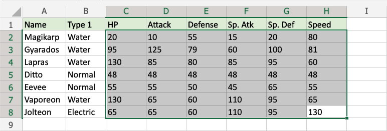
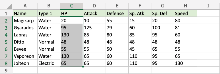
- Select the range
C2:H8for all of the stat values
- Click on the Conditional Formatting icon
 in the ribbon, from Home menu
 - Select Highlight Cell Rules from the drop-down menu
- Select Equal To… from the menu
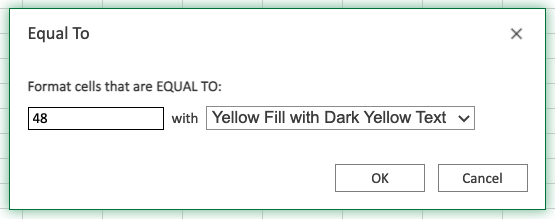
This will open a dialog box where you can specify the value and the appearance option.
- Enter
48into the input field - Select the appearance option “Yellow Fill with Dark Yellow Text” from the dropdown menu
Now, the cells with values equal to “48” will be highlighted in yellow:
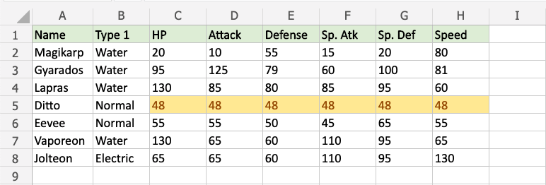
All of Ditto’s stat values are 48, so they are highlighted.
Note: You can remove the Highlight Cell Rules with Manage Rules.
Excel HCR – Greater Than
Highlight Cell Rules – Greater Than
Highlight Cell Rules is a premade type of conditional formatting in Excel used to change the appearance of cells in a range based on your specified conditions.
Greater Than… is one of the options for the condition.
Here is the Highlight Cell Rules part of the conditional formatting menu:
Highlight Cell Rule – Greater Than Example
The “Greater Than…” Highlight Cell Rule will highlight a cell with one of the appearance options based on the cell value being greater than to your specified value.
The specified value is typically a number, but it also works with a text value.
In this example, the specified value will be “65”.
You can choose any range for where the Highlight Cell Rule should apply. It can be a few cells, a single column, a single row, or a combination of multiple cells, rows and columns.
Let’s apply the rule to the HP values.
“Greater Than…” Highlight Cell Rule, step by step:
- Select the range
C2:C8for HP values
- Click on the Conditional Formatting icon in the ribbon, from Home menu
- Select Highlight Cell Rules from the drop-down menu
- Select Greater Than… from the menu
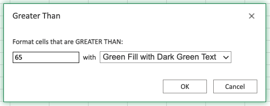
This will open a dialog box where you can specify the value and the appearance option.
- Enter
65into the input field - Select the appearance option “Green Fill with Dark Green Text” from the dropdown menu
Now, the cells with values greater than “65” will be highlighted in green:
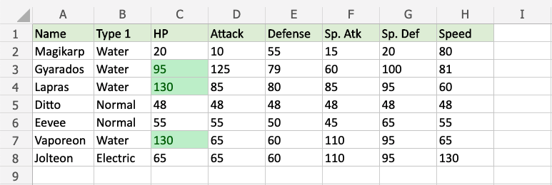
Gyarados, Lapras and Vaporeon have HP values greater than 65, so they are highlighted.
Note: Jolteon’s HP value is 65, but is not highlighted, since the rule does not include the specified value itself.
Note: You can remove the Highlight Cell Rules with Manage Rules.
Highlight Cell Rule – Greater Than Example (with Text)
The “Greater Than…” Highlight Cell Rule also works with text values.
Excel will use alphabetical order (A-Z) to highlight the text values that start with a letter that is later in the alphabet than the specified value.
In this example, the specified text value will be “Gyarados”.
You can choose any range for where the Highlight Cell Rule should apply. It can be a few cells, a single column, a single row, or a combination of multiple cells, rows and columns.
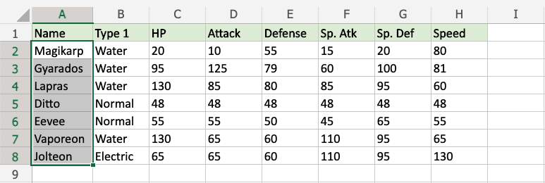
Let’s apply the rule to the Name values.
“Greater Than…” Highlight Cell Rule, step by step:
- Select the range
A2:A8for Name values
- Click on the Conditional Formatting icon in the ribbon, from Home menu
- Select Highlight Cell Rules from the drop-down menu
- Select Greater Than… from the menu
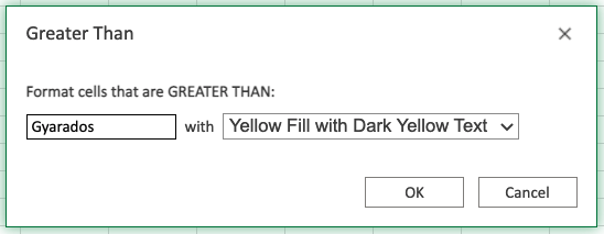
This will open a dialog box where you can specify the value and the appearance option.
- Enter
Gyaradosinto the input field - Select the appearance option “Yellow Fill with Dark Yellow Text” from the dropdown menu
Now, the cells with text values later in the alphabet than “Gyarados” will be highlighted in yellow:
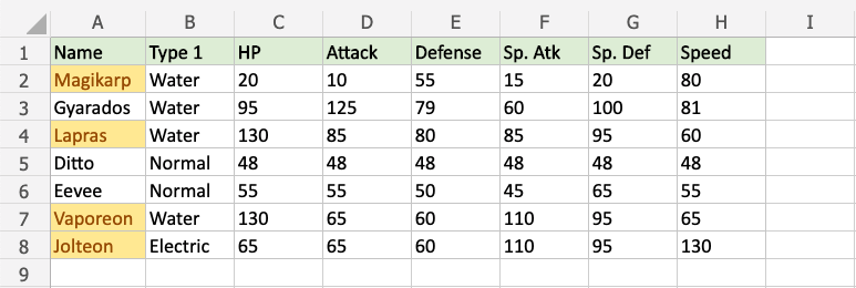
Magikarp starts with “M”, Lapras with “L”, Vaporeon with “V”, and Jolteon with “J”.
“M”, “L”, “V”, and “J” are all later in the alphabet than “G”, which Gyarados starts with, so these all are highlighted.
But, what about the rest of the letters in the text value?
Let’s see what happens if we add a fictional pokemon with a new name:
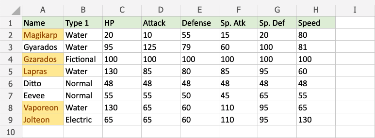
Notice that the fictional “Gzarados” is highlighted.
The Excel condition checks each letter in the specified text value from left to right.
Because the “z” in “Gzarados” comes later in the alphabet than the “y” in “Gyarados”, this is considered Greater Than and is highlighted.
Excel HCR – Less Than
Highlight Cell Rules – Less Than
Highlight Cell Rules is a premade type of conditional formatting in Excel used to change the appearance of cells in a range based on your specified conditions.
Less Than… is one of the options for the condition.
Here is the Highlight Cell Rules part of the conditional formatting menu:
Highlight Cell Rule – Less Than Example
The “Less Than…” Highlight Cell Rule will highlight a cell with one of the appearance options based on the cell value being less than to your specified value.
The specified value is typically a number, but it also works with a text value.
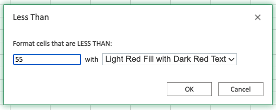
In this example, the specified value will be “55”.
You can choose any range for where the Highlight Cell Rule should apply. It can be a few cells, a single column, a single row, or a combination of multiple cells, rows and columns.
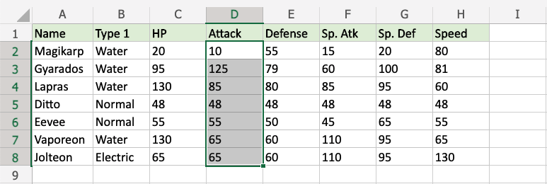
Let’s apply the rule to the Attack values.
“Less Than…” Highlight Cell Rule, step by step:
- Select the range
D2:D8for Attack values
- Click on the Conditional Formatting icon in the ribbon, from Home menu
- Select Highlight Cell Rules from the drop-down menu
- Select Less Than… from the menu
This will open a dialog box where you can specify the value and the appearance option.
- Enter
55into the input field - Select the appearance option “Light Red Fill with Dark Red Text” from the dropdown menu
Now, the cells with values less than “55” will be highlighted in red:
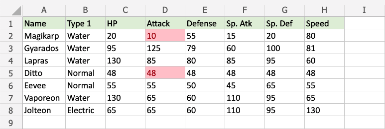
Only Magikarp and Ditto have Attack values less than 55, so these values are highlighted.
Note: Eevees’s Attack value is 55, but is not highlighted, since the rule does not include the specified value itself.
Note: You can remove the Highlight Cell Rules with Manage Rules.
Highlight Cell Rule – Less Than Example (with Text)
The “Less Than…” Highlight Cell Rule also works with text values.
Excel will use alphabetical order (A-Z) to highlight the text values that start with a letter that is earlier in the alphabet than the specified value
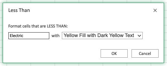
In this example, the specified text value will be “Electric”.
You can choose any range for where the Highlight Cell Rule should apply. It can be a few cells, a single column, a single row, or a combination of multiple cells, rows and columns.
Let’s apply the rule to the Type 1 values.
“Less Than…” Highlight Cell Rule, step by step:
- Select the range
B2:B8for Type 1 values

- Click on the Conditional Formatting icon in the ribbon, from Home menu
- Select Highlight Cell Rules from the drop-down menu
- Select Less Than… from the menu
This will open a dialog box where you can specify the value and the appearance option.
- Enter
Electricinto the input field - Select the appearance option “Yellow Fill with Dark Yellow Text” from the dropdown menu
Now, the cells with text values earlier in the alphabet than “Electric” will be highlighted in yellow:
Nothing seems to have changed!
Water starts with “W” and Normal starts with “N”.
“W”and “N” are all later in the alphabet than “E”, which Electric starts with, so none of these are highlighted.
Note: The specified value “Electric” itself is also not highlighted, because the rule only highlights text values that are earlier in the alphabet.
So, what about the rest of the letters in the text value?
Let’s see what happens if we add a fictional pokemon with a new Name and Type:
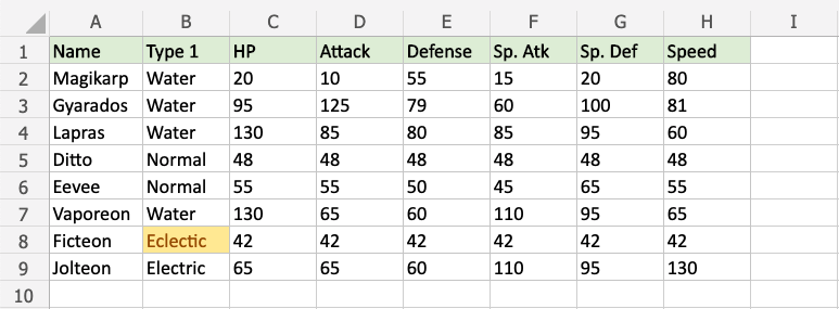
Notice that the fictional “Ficteon” has the type “Eclectic”, which is highlighted.
The Excel condition checks each letter in the specified text value from left to right.
Because the “c” in “Eclectic” comes earlier in the alphabet than the “l” in “Electric”, this is considered Less Than and is highlighted.
Excel Highlight Cell Rules – Between
Highlight Cell Rules – Between
Highlight Cell Rules is a premade type of conditional formatting in Excel used to change the appearance of cells in a range based on your specified conditions.
Between… is one of the options for the condition.
Here is the Highlight Cell Rules part of the conditional formatting menu:
Highlight Cell Rule – Between Example
The “Between…” Highlight Cell Rule will highlight a cell with one of the appearance options based on the cell value being between two specified values.
The specified values are typically numbers, but can also be text values.
In this example, the specified values will be “79” and “100”.
You can choose any range for where the Highlight Cell Rule should apply. It can be a few cells, a single column, a single row, or a combination of multiple cells, rows and columns.
Let’s apply the rule to all of the different stat values.
“Between…” Highlight Cell Rule, step by step:
- Select the range
C2:H8for all of the stat values
- Click on the Conditional Formatting icon in the ribbon, from Home menu
- Select Highlight Cell Rules from the drop-down menu
- Select Between… from the menu
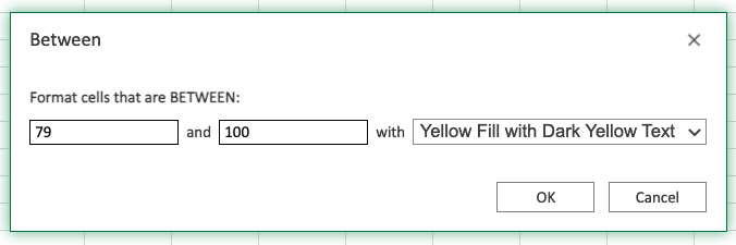
This will open a dialog box where you can specify the value and the appearance option.
- Enter
79and100into the input fields - Select the appearance option “Yellow Fill with Dark Yellow Text” from the dropdown menu
Now, the cells with values between “79” and “100” will be highlighted in yellow:
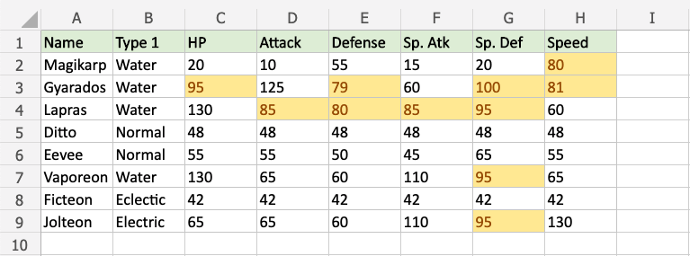
Notice that Gyarados’ Defense and Special Defense, which are 79 and 100, are highlighted.
The Between… condition includes the specified values. This is different from the Greater Than… and Less Than… conditions, which do not include the specified values.
Note: You can remove the Highlight Cell Rules with Manage Rules.
Excel HCR – Equal To
Highlight Cell Rules – Equal To
Highlight Cell Rules is a premade type of conditional formatting in Excel used to change the appearance of cells in a range based on your specified conditions.
Equal To… is one of the options for the condition.
Here is the Highlight Cell Rules part of the conditional formatting menu:
Highlight Cell Rule – Equal To Example (with Numbers)
The “Equal To…” Highlight Cell Rule will highlight a cell with one of the appearance options based on the cell value being equal to your specified value.
The specified value could be a particular number or particular text.
In this example, the specified value will be “48”.
You can choose any range for where the Highlight Cell Rule should apply. It can be a few cells, a single column, a single row, or a combination of multiple cells, rows and columns.
Let’s apply the rule to all of the different stat values.
“Equal To…” Highlight Cell Rule, step by step:
- Select the range
C2:H8for all of the stat values
- Click on the Conditional Formatting icon in the ribbon, from Home menu
- Select Highlight Cell Rules from the drop-down menu
- Select Equal To… from the menu
This will open a dialog box where you can specify the value and the appearance option.
- Enter
48into the input field - Select the appearance option “Yellow Fill with Dark Yellow Text” from the dropdown menu
Now, the cells with values equal to “48” will be highlighted in yellow:
All of Ditto’s stat values are 48, so they are highlighted.
Note: You can remove the Highlight Cell Rules with Manage Rules.
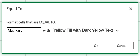
Highlight Cell Rule – Equal To Example (with Text)
The “Equal To…” Highlight Cell Rule also works with text values.
In this example, the specified text value will be “Magikarp”.
You can choose any range for where the Highlight Cell Rule should apply. It can be a few cells, a single column, a single row, or a combination of multiple cells, rows and columns.
Let’s apply the rule to the Name values.
“Equal To…” Highlight Cell Rule, step by step:
- Select the range
A2:A8for Name values
- Click on the Conditional Formatting icon in the ribbon, from Home menu
- Select Highlight Cell Rules from the drop-down menu
- Select Equal To… from the menu
This will open a dialog box where you can specify the value and the appearance option.
- Enter
Magikarpinto the input field - Select the appearance option “Yellow Fill with Dark Yellow Text” from the dropdown menu
Now, the cells with text values equal to “Magikarp” will be highlighted in yellow:
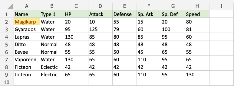
Note: The Equal To… Highlight Cell Rule will highlight cells that exactly match the specified value.
You can use the Text That Contains rule for highlighting cells that have values with any part matching the specified value.
Excel HCR – Text That Contains
Highlight Cell Rules – Text That Contains
Highlight Cell Rules is a premade type of conditional formatting in Excel used to change the appearance of cells in a range based on your specified conditions.
Text That Contains… is one of the options for the condition.
Here is the Highlight Cell Rules part of the conditional formatting menu:
Highlight Cell Rule – Text That Contains Example (with Text)
The “Text That Contains…” Highlight Cell Rule will highlight a cell with one of the appearance options based on a part of the cell value containing your specified value.
The specified value is typically text, but also works with a numerical value.
In this example, the specified value will be “Pidge”.
You can choose any range for where the Highlight Cell Rule should apply. It can be a few cells, a single column, a single row, or a combination of multiple cells, rows and columns.
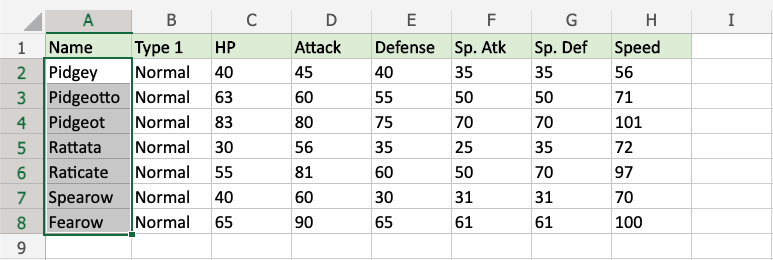
Let’s apply the rule to the Name values.
“Text That Contains…” Highlight Cell Rule, step by step:
- Select the range
A2:A8for the Name values
- Click on the Conditional Formatting icon in the ribbon, from Home menu
- Select Highlight Cell Rules from the drop-down menu
- Select Text That Contains… from the menu
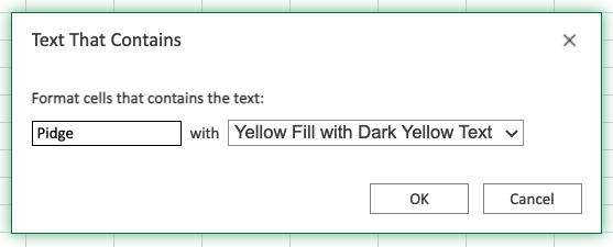
This will open a dialog box where you can specify the value and the appearance option.
- Enter
Pidgeinto the input field - Select the appearance option “Yellow Fill with Dark Yellow Text” from the dropdown menu
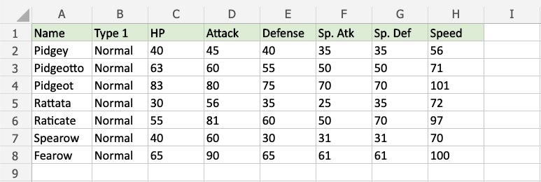
Now, the cells with values Text That Contains “Pidge” will be highlighted in yellow:
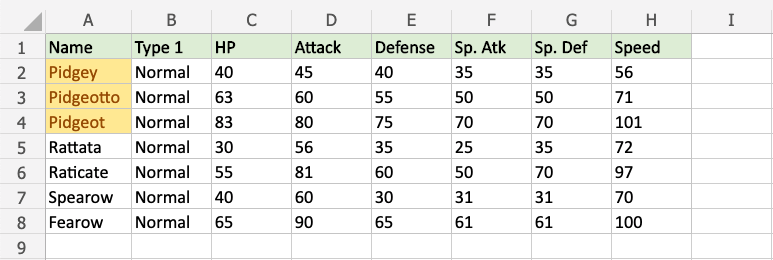
The names “Pidgey”, “Pidgeot”, and “Pidgeotto” all start with “Pidge”, so all these cells are highlighted.
Note: The Text That Contains rule works with any part of the cell values.
Like in the example below:
Highlight Cell Rule – Text That Contains Example 2 (with Text)
The “Text That Contains…” Highlight Cell Rule will highlight a cell with one of the appearance options based on a part of the cell value containing your specified value.
The specified value is typically text, but also works with a numerical value.
In this example, the specified value will be “row”.
You can choose any range for where the Highlight Cell Rule should apply. It can be a few cells, a single column, a single row, or a combination of multiple cells, rows and columns.
Let’s apply the rule to the Name values.
“Text That Contains…” Highlight Cell Rule, step by step:
- Select the range
A2:A8for the Name values
- Click on the Conditional Formatting icon in the ribbon, from Home menu
- Select Highlight Cell Rules from the drop-down menu
- Select Text That Contains… from the menu
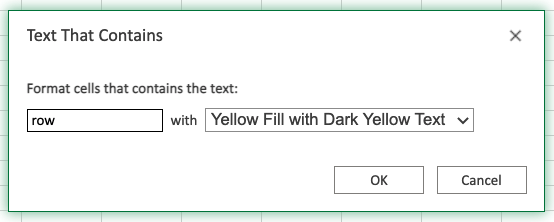
This will open a dialog box where you can specify the value and the appearance option.
- Enter
rowinto the input field - Select the appearance option “Yellow Fill with Dark Yellow Text” from the dropdown menu
Now, the cells with values Text That Contains “row” will be highlighted in yellow:
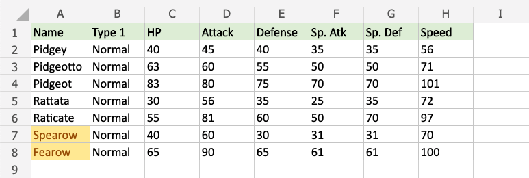
The names “Spearow” and “Fearow” both end with “row”, so both cells are highlighted.
Note: You can remove the Highlight Cell Rules with Manage Rules.
Highlight Cell Rule – Text That Contains Example (with Numbers)
The “Text That Contains…” Highlight Cell Rule also works with numbers.
In this example, the specified text value will be “7”.
You can choose any range for where the Highlight Cell Rule should apply. It can be a few cells, a single column, a single row, or a combination of multiple cells, rows and columns.
Let’s apply the rule to all the different stat values.
“Text That Contains…” Highlight Cell Rule, step by step:
- Select the range
C2:H8for all the stat values
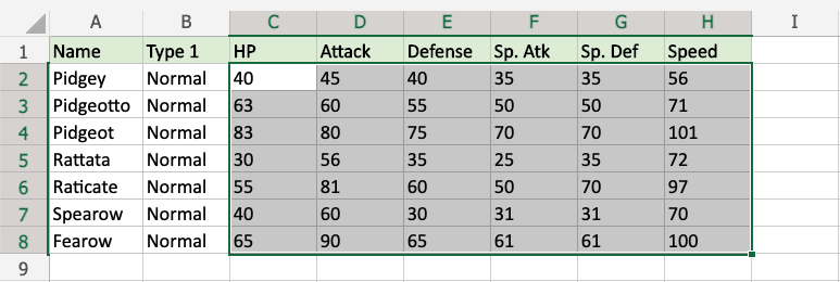
- Click on the Conditional Formatting icon in the ribbon, from Home menu
- Select Highlight Cell Rules from the drop-down menu
- Select Text That Contains… from the menu
This will open a dialog box where you can specify the value and the appearance option.
- Enter
7into the input field - Select the appearance option “Green Fill with Dark Green Text” from the dropdown menu

Now, the cells with values That Contains “7” anywhere will be highlighted in green:
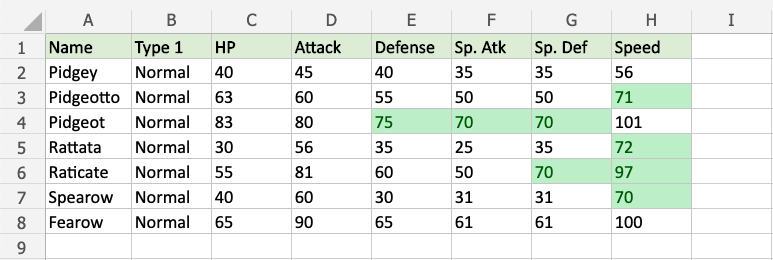
Note: The Text That Contains… Highlight Cell Rule will highlight cells that have values with any part matching the specified value.
You can use the Equal To… rule for highlighting cells that exactly match the specified value.
Excel HCR – A Date Occurring
Highlight Cell Rules – A Date Occurring
Highlight Cell Rules is a premade type of conditional formatting in Excel used to change the appearance of cells in a range based on your specified conditions.
A Date Occurring… is one of the options for the condition.
Here is the Highlight Cell Rules part of the conditional formatting menu:
Highlight Cell Rule – A Date Occurring Example
The “A Date Occurring…” Highlight Cell Rule will highlight a cell with one of the appearance options based on the cell value relative to a specified time frame.
The time frame can be:
- Yesterday
- Today
- Tomorrow
- In the last 7 days
- Last Week
- This Week
- Next Week
- Last Month
- This Month
- Next Month
In this example, the specified time frame will be “next month”.
You can choose any range for where the Highlight Cell Rule should apply. It can be a few cells, a single column, a single row, or a combination of multiple cells, rows and columns.
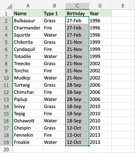
Let’s apply the rule to the Birthday values.
“A Date Occurring…” Highlight Cell Rule, step by step:
- Select the range
C2:C19for the Birthday values
- Click on the Conditional Formatting icon in the ribbon, from Home menu
- Select Highlight Cell Rules from the drop-down menu
- Select A Date Occurring… from the menu
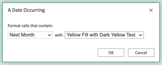
This will open a dialog box where you can specify the value and the appearance option.
- Select “Next Month” from the dropdown menu
- Select the appearance option “Yellow Fill with Dark Yellow Text” from the dropdown menu
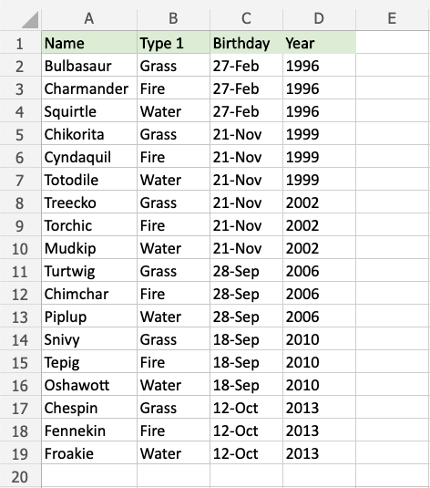
Now, the cells with values A Date Occurring next month will be highlighted in yellow:
Note: In this example, the next month happens to be September.
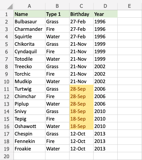
Turtwig, Chimchar, Piplup, Snivy, Tepig, and Oshawott all have birthdays in September, so their cells are highlighted.
Note: You can remove the Highlight Cell Rules with Manage Rules.
Excel HCR – Duplicate and Unique Values
Highlight Cell Rules – Duplicate and Unique Values
Highlight Cell Rules is a premade type of conditional formatting in Excel used to change the appearance of cells in a range based on your specified conditions.
Duplicate Values.. is one of the options for the condition, and can check for both duplicate and unique values.
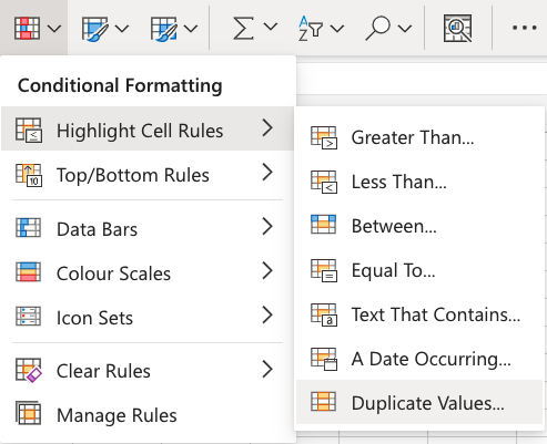
Here is the Highlight Cell Rules part of the conditional formatting menu:
Highlight Cell Rule – Duplicate Value Example
The “Duplicate Values…” Highlight Cell Rule will highlight a cell with one of the appearance options based on the cell value being the same as other cells in the range.
You can choose any range for where the Highlight Cell Rule should apply. It can be a few cells, a single column, a single row, or a combination of multiple cells, rows and columns.
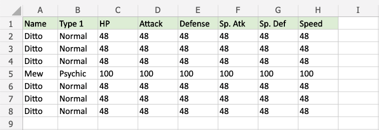
Let’s apply the rule to all of the cell values.
“Duplicate Values…” Highlight Cell Rule, step by step:
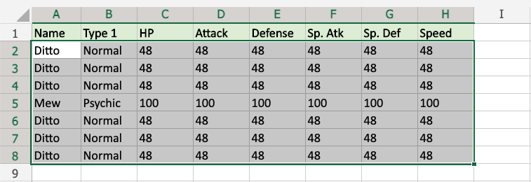
- Select the range
A2:H8
- Click on the Conditional Formatting icon in the ribbon, from Home menu
- Select Highlight Cell Rules from the drop-down menu
- Select Duplicate Values… from the menu
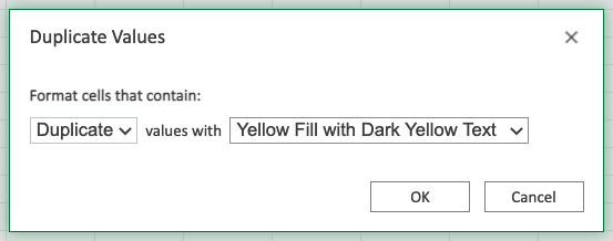
This will open a dialog box where you can specify the value and the appearance option.
- Select Duplicate
- Select the appearance option “Yellow Fill with Dark Yellow Text” from the dropdown menu
Now, all the cells in the range that have the same value as another cell are highlighted in yellow:
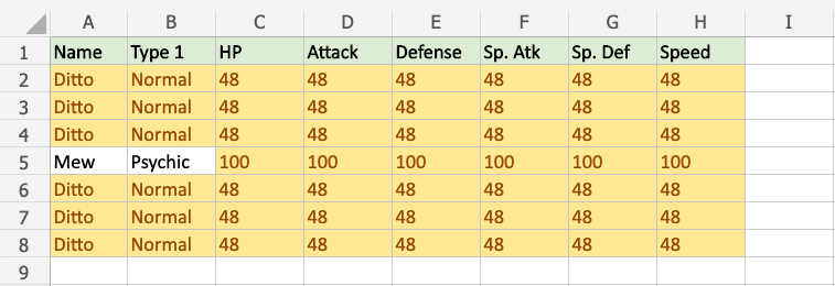
All of Ditto’s stat values are 48 and all of Mew’s stat values are 100, so they are all highlighted.
All of the Dittos and all of the Normal Type values are also highlighted.
Note: You can remove the Highlight Cell Rules with Manage Rules.
Highlight Cell Rule – Unique Value Example
The “Duplicate Values…” Highlight Cell Rule can also find and highlight Unique Values.
Let’s apply this to the same set of data:
You can choose any range for where the Highlight Cell Rule should apply. It can be a few cells, a single column, a single row, or a combination of multiple cells, rows and columns.
Let’s apply the rule to all of the cell values.
“Duplicate Values…” Highlight Cell Rule, step by step:
- Select the range
A2:H8
- Click on the Conditional Formatting icon in the ribbon, from Home menu
- Select Highlight Cell Rules from the drop-down menu
- Select Duplicate Values… from the menu
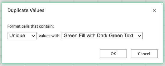
This will open a dialog box where you can specify the value and the appearance option.
- Select Unique from the dropdown menu
- Select the appearance option “Green Fill with Dark Green Text” from the dropdown menu
Now, the cells with unique values will be highlighted in green:
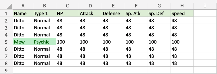
Mew and Psychic only appears once in the range, so these values are highlighted.
Note: You can remove the unwanted duplicates from a table with Removing Duplicate Function.